To celebrate the publication of our MuZero paper in [cached]Nature ([cached]full-text), I've written a high level description of the MuZero algorithm. My focus here is to give you an intuitive understanding and general overview of the algorithm; for the full details please read the paper. Please also see our [cached]official DeepMind blog post, it has great animated versions of the figures!
MuZero is a very exciting step forward - it requires no special knowledge of game rules or environment dynamics, instead learning a model of the environment for itself and using this model to plan. Even though it uses such a learned model, MuZero preserves the full planning performance of AlphaZero - opening the door to applying it to many real world problems!
It's all just statistics
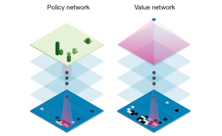
MuZero is a machine learning algorithm, so naturally the first thing to understand is how it uses neural networks. From AlphaGo and AlphaZero, it inherited the use of policy and value networks1:
Both the policy and the value have a very intuitive meaning:
-
The policy, written $p(s, a)$, is a probability distribution over all actions $a$ that can be taken in state $s$. It estimates which action is likely to be the optimal action. The policy is similar to the first guess for a good move that a human player has when quickly glancing at a game.
-
The value $v(s)$ estimates the probability of winning from the current state $s$: averaging over all possible future possibilities, weighted by how likely they are, in what fraction of them would the current player win?
Each of these networks on their own is already very powerful: If you only have a policy network, you could simply always play the move it predicts as most likely and end up with a very decent player. Similarly, given only a value network, you could always choose the move with the highest value. However, combining both estimates leads to even better results.
Planning to Win
Similar to AlphaGo and AlphaZero before it, MuZero uses Monte Carlo Tree Search2, short MCTS, to aggregate neural network predictions and choose actions to apply to the environment.
MCTS is an iterative, best-first tree search procedure. Best-first means expansion of the search tree is guided by the value estimates in the search tree. Compared to classic methods such as breadth-first (expand the entire tree up to a fixed depth before searching deeper) or depth-first (consecutively expand each possible path until the end of the game before trying the next), best-first search can take advantage of heuristic estimates (such as neural networks) to find promising solutions even in very large search spaces.
MCTS has three main phases: simulation, expansion and backpropagation. By repeatedly executing these phases, MCTS incrementally builds a search tree over future action sequences one node at a time. In this tree, each node is a future state, while the edges between nodes represent actions leading from one state to the next.
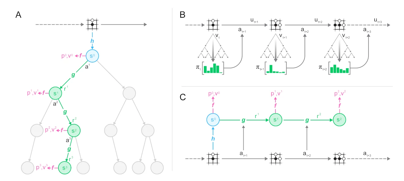
Before we dive into the details, let me introduce a schematic representation of such a search tree, including the neural network predictions made by MuZero:
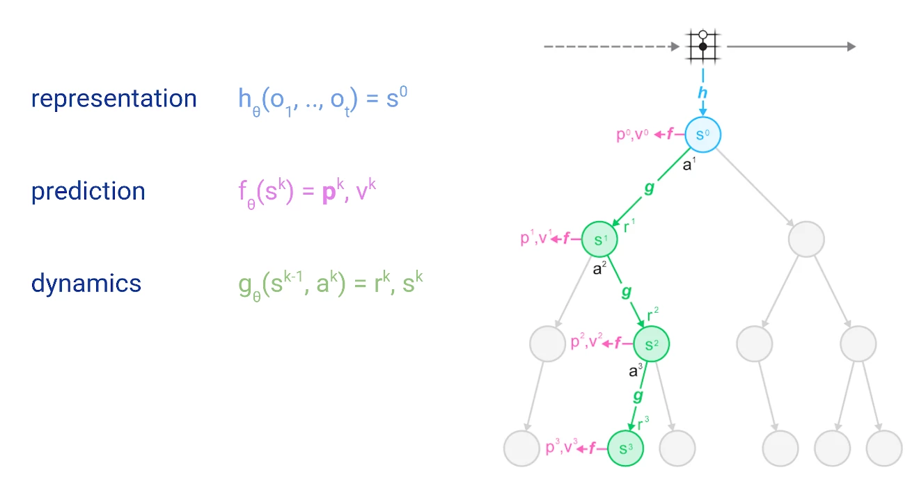
Circles represent nodes of the tree, which correspond to states in the environment. Lines represent actions, leading from one state to the next. The tree is rooted at the top, at the current state of the environment - represented by a schematic Go board. We will cover the details of representation, prediction and dynamics functions in a later section.
Simulation always starts at the root of the tree (light blue circle at the top of the figure), the current position in the environment or game. At each node (state $s$), it uses a scoring function $U(s, a)$ to compare different actions $a$ and chose the most promising one. The scoring function used in MuZero would combine a prior estimate $p(s, a)$ with the value estimate for $v(s, a)$:
$$ U(s, a) = v(s, a) + c \cdot p(s, a) $$
where $c$ is a scaling factor3 that ensures that the influence of the prior diminishes as our value estimate becomes more accurate.
Each time an action is selected, we increment its associated visit count $n(s, a)$, for use in the UCB scaling factor $c$ and for later action selection.
Simulation proceeds down the tree until it reaches a leaf that has not yet been expanded; at this point the neural network is used to evaluate the node. Evaluation results (prior and value estimates) are stored in the node.
Expansion: Once a node has reached a certain number of evaluations, it is marked as "expanded". Being expanded means that children can be added to a node; this allows the search to proceed deeper. In MuZero, the expansion threshold is 1, i.e. every node is expanded immediately after it is evaluated for the first time. Higher expansion thresholds can be useful to collect more reliable statistics4 before searching deeper.
Backpropagation: Finally, the value estimate from the neural network evaluation is propagated back up the search tree; each node keeps a running mean of all value estimates below it. This averaging process is what allows the UCB formula to make increasingly accurate decisions over time, and so ensures that the MCTS will eventually converge to the best move.
Intermediate Rewards
The astute reader may have noticed that the figure above also includes the prediction of a quantity $r$. Some domains, such as board games, only provide feedback at the end of an episode (e.g. a win/loss result); they can be modeled purely through value estimates. Other domains however provide more frequent feedback, in the general case a reward $r$ is observed after every transition from one state to the next.
Directly modeling this reward through a neural network prediction and using it in the search is advantageous. It only requires a slight modification to the UCB formula:
$$ U(s, a) = r(s, a) + \gamma \cdot v(s') + c \cdot p(s, a) $$
where $r(s, a)$ is the reward observed in transitioning from state $s$ by choosing action $a$, and $\gamma$ is a discount factor that describes how much we care about future rewards.
Since in general rewards can have arbitrary scale, we further normalize the combined reward/value estimate to lie in the interval $[0, 1]$ before combining it with the prior:
$$ U(s, a) = \frac{r(s, a) + \gamma \cdot v(s') - q_{min}}{q_{max} - q_{min}} + c \cdot p(s, a) $$
where $q_{min}$ and $q_{max}$ are the minimum and maximum $r(s, a) + \gamma \cdot v(s')$ estimates observed across the search tree.
Episode Generation
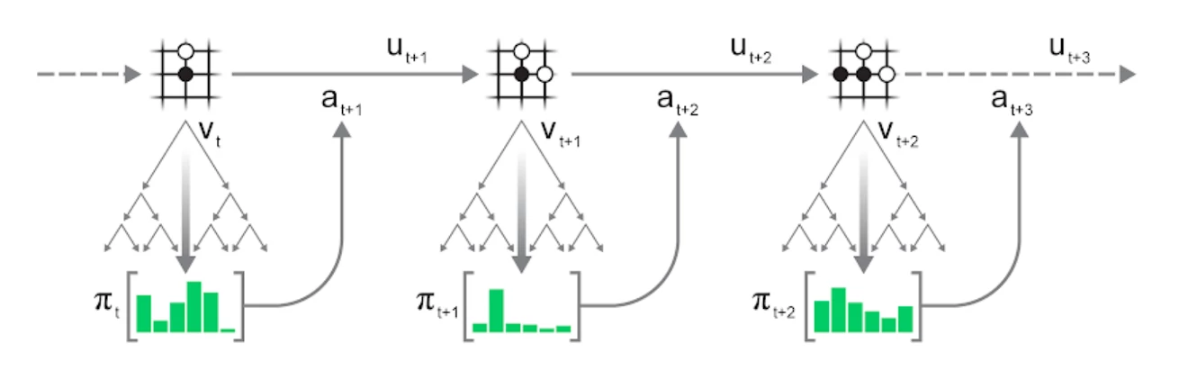
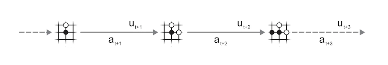
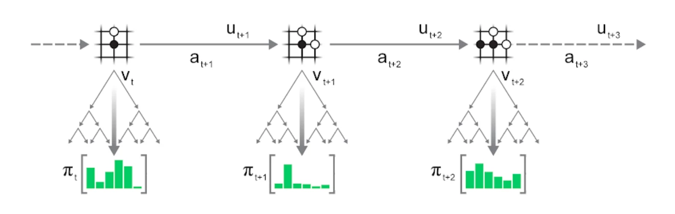
The MCTS procedure described above can be applied repeatedly to play entire episodes:
- Run a search in the current state $s_t$ of the environment.
- Select an action $a_{t+1}$ according to the statistics $\pi_t$ of the search.
- Apply the action to the environment to advance to the next state $s_{t+1}$ and observe reward $u_{t+1}$.
- Repeat until the environment terminates.
Action selection can either be greedy - select the action with the most visits - or exploratory: sample action $a$ proportional to its visit count $n(s, a)$, potentially after applying some temperature $t$ to control the degree of exploration:
$$ p(a) = {\left( \frac{n(s, a)}{\sum_b n(s, b)} \right)}^{1/t} $$
For $t = 0$, we recover greedy action selection; $t = \inf$ is equivalent to sampling actions uniformly.
Training
Now that we know how to run MCTS to select actions, interact with the environment and generate episodes, we can turn towards training the MuZero model.
We start by sampling a trajectory and a position within it from our dataset, then we unroll the MuZero model alongside the trajectory:
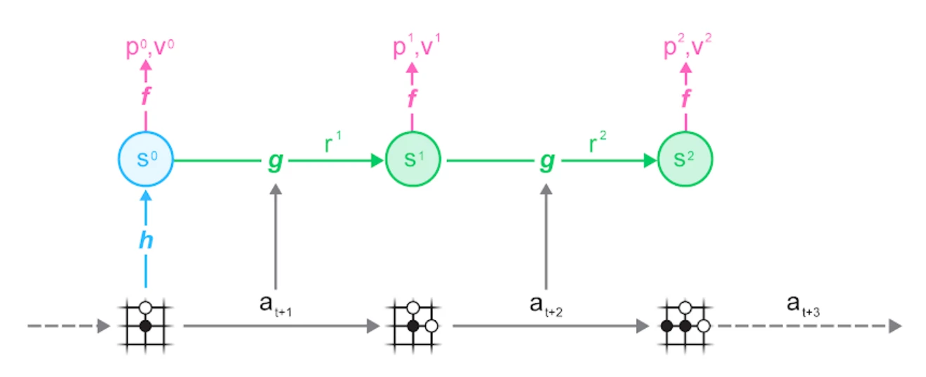
You can see the three parts of the MuZero algorithm in action:
- the representation function $h$ maps from a set of observations (the schematic Go board) to the hidden state $s$ used by the neural network
- the dynamics function $g$ maps from a state $s_t$ to the next state $s_{t+1}$ based on an action $a_{t+1}$. It also estimates the reward $r_t$ observed in this transition. This is what allows the learned model to be rolled forward inside the search.
- the prediction function $f$ makes estimates for policy $p_t$ and value $v_t$ based on a state $s_t$. These are the estimates used by the UCB formula and aggregated in the MCTS.
The observations and actions used as input to the network are taken from this trajectory; similarly the prediction targets for policy, value and reward are the ones stored with the trajectory when it was generated.
You can see this alignment between episode generation (B) and training (C) even more clearly in the full figure:
Specifically, the training losses for the three quantities estimated by MuZero are:
- policy: cross-entropy between MCTS visit count statistics and policy logits from the prediction function.
- value: cross-entropy or mean squared error between discounted sum of N rewards + stored search value or target network estimate and value from the prediction function5.
- reward: cross-entropy between reward observed in the trajectory and dynamics function estimate.
Reanalyse
Having examined the core MuZero training, we are ready to take a look at the technique that allows us to leverage the search to achieve massive data-efficiency improvements: Reanalyse.
In the course of normal training, we generate many trajectories (interactions with the environment) and store them in our replay buffer for training. Can we get more mileage out of this data?
Unfortunately, since this is stored data, we cannot change the states, actions or received rewards - this would require resetting the environment to an arbitrary state and continuing from there. Possible in The Matrix, but not in the real world.
Luckily, it turns out that we don't need to - using existing inputs with fresh, improved labels is enough for continued learning. Thanks to MuZero's learned model and the MCTS, this is exactly what we can do:
We keep the saved trajectory (observations, actions and rewards) as is and instead only re-run the MCTS. This generates fresh search statistics, providing us with new targets for the policy and value prediction.
In the same way that searching with an improved network results in better search statistics when interacting with the environment directly, re-running the search with an improved network on saved trajectories also results in better search statistics, allowing for repeated improvements using the same trajectory data.
Reanalyse fits naturally into the MuZero training loop. Let's start with the normal training loop:
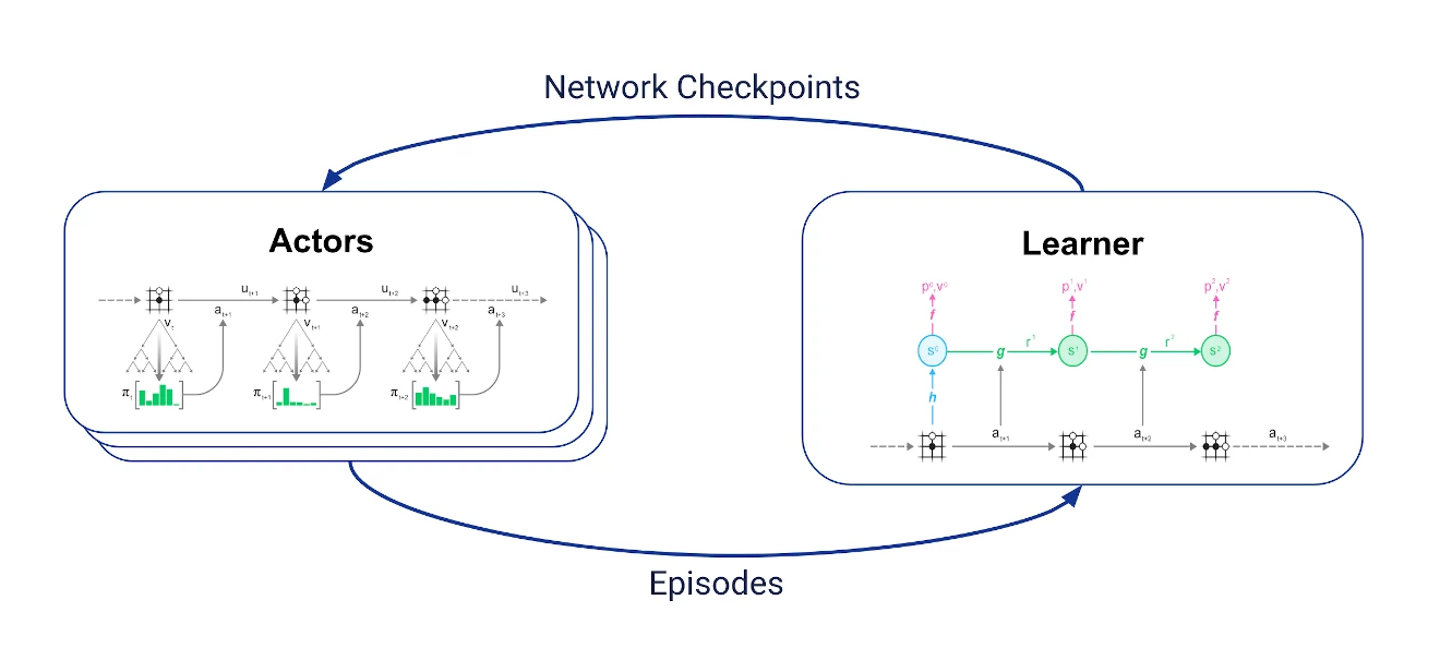
We have two sets of jobs that communicate with each other asynchronously:
- a learner that receives the latest trajectories, keeps the most recent of these in a replay buffer and uses them to perform the training algorithm described above.
- multiple actors which periodically fetch the latest network checkpoint from the learner, use the network in MCTS to select actions and interact with the environment to generate trajectories.
To implement reanalyse, we introduce two jobs:
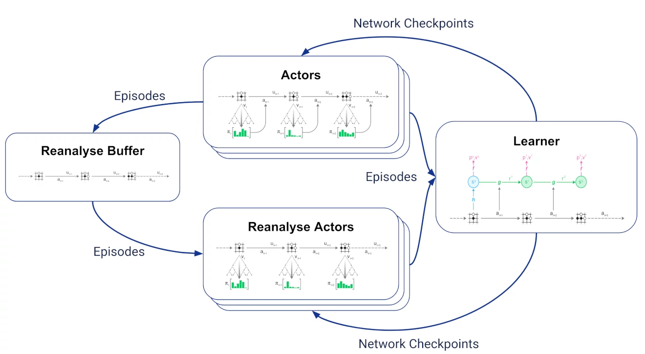
- a reanalyse buffer that receives all trajectories generated by the actors and keeps the most recent ones.
- multiple reanalyse actors 6 that sample stored trajectories from the reanalyse buffer, re-run MCTS using the latest network checkpoints from the learner and send the resulting trajectories with updated search statistics to the learner.
For the learner, "fresh" and reanalysed trajectories are indistinguishable; this makes it very simple to vary the proportion of fresh vs reanalysed trajectories.
What's in a name?
MuZero's name is of course based on AlphaZero - keeping the Zero to indicate that it was trained without imitating human data, and replacing Alpha with Mu to signify that it now uses a learned model to plan.
Digging a little deeper, we find that Mu is rich in meaning:
- [cached]夢, which can be read as mu in Japanese, means 'dream' - just like MuZero uses the learned model to imagine future scenarios.
- the greek letter μ, pronounced mu, can also stand for the learned model.
- [cached]無, pronunced mu in Japanese, means 'nothing' - doubling down on the notion of learning from scratch: not just no human data to imitate, but not even provided with the rules.
Final Words
I hope this summary of MuZero was useful!
If you are interested in more details, start with the [cached]full paper (pdf). I also gave talks about MuZero at [cached]NeurIPS ([cached]poster) and most [cached]recently at ICAPS. Also see the up-to-date [cached]pseudocode.
Let me finish by linking some articles, blog posts and GitHub projects from other researchers that I found interesting:
- [cached]A Simple Alpha(Go) Zero Tutorial
- [cached]MuZero General implementation
- [cached]How To Build Your Own MuZero AI Using Python
-
For simplicity, in MuZero both of these predictions are made by a single network, the prediction function. ↩
-
Introduced by Rémi Coulom in Efficient Selectivity and Backup Operators in Monte-Carlo Tree Search, 2006, MCTS lead to a major improvement in the playing strength of all Go playing programs. "Monte Carlo" in MCTS refers to [cached]random playouts used in Go playing programs at the time, estimating the chance of winning in a particular position by playing random moves until the end of the game. ↩
-
The exact scaling used in MuZero is $\frac{\sqrt{\sum_b n(s, b)}}{1 + n(s, a)} \cdot (c_1 + \log(\frac{\sum_b n(s, b) + c_2 + 1}{c_2}))$, where $n(s, a)$ are the number of visits for action $a$ from state $s$, and $c_1 = 1.25$ and $c_2 = 19652$ are constants to influence the important of the prior relative to the value estimate. Note that for $c_2 \gg n$, the exact value of $c_2$ is not important and the $log$ term becomes 0. In this case, the formula simplifies to $c_1 \cdot \frac{\sqrt{\sum_b n(s, b)}}{1 + n(s, a)}$ ↩
-
This is most useful when using stochastic evaluation functions such as random rollouts as used by many Go programs before AlphaGo. If the evaluation function is deterministic (such as a standard neural network), evaluating the same nodes multiple times is less useful. ↩
-
For board games, the discount $\gamma$ is 1 and the number of TD steps infinite, so this is just prediction of the Monte Carlo return (winner of the game). ↩
-
In our implementation of MuZero, there is no separate set of actors for reanalyse: We have a single set of actors which decide at the start of each episode whether to start a fresh trajectory interacting with the environment or to reanalyse a stored trajectory. ↩